4 Using TMB
We are now ready to present the main TMB code for calculating the negative log-likelihood of an HMM.
4.1 Likelihood function
The function is defined in code/poi_hmm.cpp and imports the utility functions defined in functions/utils.cpp.
#include <TMB.hpp>
#include "../functions/utils.cpp"

// Likelihood for a poisson hidden markov model.
template<class Type>
Type objective_function<Type>::operator() ()
{

  // Data
  DATA_VECTOR(x);          // timeseries vector
  DATA_INTEGER(m);         // Number of states m

  // Parameters
  PARAMETER_VECTOR(tlambda);     // conditional log_lambdas's
  PARAMETER_VECTOR(tgamma);      // m(m-1) working parameters of TPM

  // Uncomment only when using a non-stationary distribution
  //PARAMETER_VECTOR(tdelta);    // transformed stationary distribution,

  // Transform working parameters to natural parameters:
  vector<Type> lambda = tlambda.exp();
  matrix<Type> gamma = gamma_w2n(m, tgamma);

  // Construct stationary distribution
  vector<Type> delta = stat_dist(m, gamma);
  // If using a non-stationary distribution, use this instead
  //vector<Type> delta = delta_w2n(m, tdelta);

  // Get number of timesteps (n)
  int n = x.size();

  // Evaluate conditional distribution: Put conditional
  // probabilities of observed x in n times m matrix
  // (one column for each state, one row for each datapoint):
  matrix<Type> emission_probs(n, m);
  matrix<Type> row1vec(1, m);
  row1vec.setOnes();
  for (int i = 0; i < n; i++) {
    if (x[i] != x[i]) { // f != f returns true if and only if f is NaN.
      // Replace missing values (NA in R, NaN in C++) with 1
      emission_probs.row(i) = row1vec;
    }
    else {
      emission_probs.row(i) = dpois(x[i], lambda, false);
    }
  }

  // Corresponds to (Zucchini et al., 2016, p 333)
  matrix<Type> foo, P;
  Type mllk, sumfoo, lscale;

  foo = (delta * vector<Type>(emission_probs.row(0))).matrix();
  sumfoo = foo.sum();
  lscale = log(sumfoo);
  foo.transposeInPlace();
  foo /= sumfoo;
  for (int i = 2; i <= n; i++) {
    P = emission_probs.row(i - 1);
    foo = ((foo * gamma).array() * P.array()).matrix();
    sumfoo = foo.sum();
    lscale += log(sumfoo);
    foo /= sumfoo;
  }
  mllk = -lscale;

  // Use adreport on variables for which we want standard errors
  ADREPORT(lambda);
  ADREPORT(gamma);
  ADREPORT(delta);

  // Variables we need for local decoding and in a convenient format
  REPORT(lambda);
  REPORT(gamma);
  REPORT(delta);
  REPORT(n);
  REPORT(emission_probs);
  REPORT(mllk);

  return mllk;
}
Note that we use similar names as to the TMB side.
4.2 Optimization
Before we can fit the model, we need to load some necessary packages and data files. We also need to compile the C++ code and load the functions into our working environment in R.
- We start by compiling the
C++code for computing the likelihood and its gradients. Once it is compiled, we can load the TMB likelihood object intoR– making it available fromR.
# Load TMB and optimization packages
library(TMB)
# Run the C++ file containing the TMB code
TMB::compile("code/poi_hmm.cpp")
# Load it
dyn.load(dynlib("code/poi_hmm"))
Next, we need to load the necessary packages and the utility R functions.
# Load the parameter transformation function
source("functions/utils.R")- The data are part of a large data set collected with the “Track Your Tinnitus” (TYT) mobile application, a detailed description of which is presented in Pryss, Reichert, Langguth, et al. (2015) and Pryss, Reichert, Herrmann, et al. (2015). We analyze 87 successive days of the “arousal” variable, which is measured on a discrete scale. Higher values correspond to a higher degree of excitement, lower values to a more calm emotional state (for details, see Probst et al. 2016). The data can be loaded by a simple call.
load("data/tinnitus.RData")Figure 4.1 presents the raw data in the Table below, which are also available for download at data/tinnitus.RData.
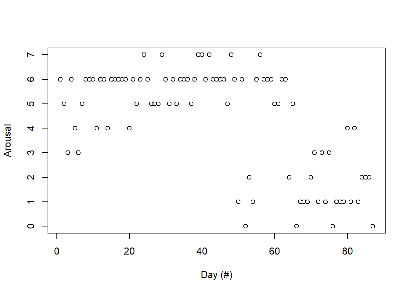
Figure 4.1: Plot of observations from TYT app data for 87 succesive days.
- Initialization of the number of states and starting (or initial) values for the optimization.
First, the number of states needs to be determined. As explained by Pohle et al. (2017a), Pohle et al. (2017b), and Zucchini, MacDonald, and Langrock (2016, sec. 6) (to name only a few), usually one would first fit models with a different number of states. Then, these models are evaluated e.g. by means of model selection criteria (as carried out by Leroux and Puterman 1992) or prediction performance (Celeux and Durand 2008).
As shown in the appendix, the model selection procedure shows that both AIC and BIC prefer a two-state model over a Poisson regression and over a model with three or four states. Consequently, we focus on the two-state model in the following.
The list object TMB_data contains the data and the number of states.
# Model with 2 states
m <- 2
TMB_data <- list(x = tinn_data, m = m)
Secondly, initial values for the optimization procedure need to be defined. Although we will apply unconstrained optimization, we initialize the natural parameters, because this is much more intuitive and practical than handling the working parameters.
# Generate initial set of parameters for optimization
lambda <- c(1, 3)
gamma <- matrix(c(0.8, 0.2,
0.2, 0.8), byrow = TRUE, nrow = m)- Transformation from natural to working parameters
The previously created initial values are transformed and stored in the list parameters for the optimization procedure.
# Turn them into working parameters
parameters <- pois.HMM.pn2pw(m, lambda, gamma)- Creation of the
TMBnegative log-likelihood function with its derivatives
This object, stored as obj_tmb requires the data, the initial values, and the previously created DLL as input.
Setting argument silent = TRUE disables tracing information and is only used here to avoid excessive output.
obj_tmb <- MakeADFun(TMB_data, parameters,
                     DLL = "poi_hmm", silent = TRUE)
This object also contains the previously defined initial values as a vector (par) rather than a list.
The negative log-likelihood (fn), its gradient (gr), and Hessian (he) are functions of the parameters (in vector form) while the data are considered fixed.
These functions are available to the user and can be evaluated for instance at the initial parameter values:
obj_tmb$par
##   tlambda   tlambda    tgamma    tgamma
##  0.000000  1.098612 -1.386294 -1.386294
obj_tmb$fn(obj_tmb$par)
## [1] 228.3552
obj_tmb$gr(obj_tmb$par)
##          [,1]      [,2]     [,3]      [,4]
## [1,] -3.60306 -146.0336 10.52832 -1.031706
obj_tmb$he(obj_tmb$par)
##           [,1]       [,2]       [,3]       [,4]
## [1,]  1.902009  -5.877900 -1.3799682  2.4054017
## [2,] -5.877900 188.088247 -4.8501589  2.3434284
## [3,] -1.379968  -4.850159  9.6066700 -0.8410438
## [4,] 2.405402 2.343428 -0.8410438 0.7984216- Execution of the optimization
For this step we rely again on the optimizer implemented in the nlminb function.
The arguments, i.e.~ initial values for the parameters and the function to be optimized, are extracted from the previously created TMB object.
mod_tmb <- nlminb(start = obj_tmb$par, objective = obj_tmb$fn)
# Check that it converged successfully
mod_tmb$convergence == 0
## [1] TRUE
It is noteworthy that various alternatives to nlminb exist.
Nevertheless, we focus on this established optimization routine because of its high speed of convergence.
- Obtaining ML estimates
Obtaining the ML estimates of the natural parameters together with their standard errors is possible by using the previously introduced command sdreport.
Recall that this requires the parameters of interest to be treated by the ADREPORT statement in the C++ part. It should be noted that the presentation of the set of parameters gamma below results from a column-wise representation of the TPM.
summary(sdreport(obj_tmb, par.fixed = mod_tmb$par), "report")
##          Estimate Std. Error
## lambda 1.63641070 0.27758294
## lambda 5.53309626 0.31876141
## gamma  0.94980192 0.04374682
## gamma  0.02592209 0.02088689
## gamma  0.05019808 0.04374682
## gamma  0.97407791 0.02088689
## delta  0.34054163 0.23056401
## delta  0.65945837 0.23056401
Note that the table above also contains estimation results for \({\boldsymbol\delta}\) and accompanying standard errors, although \({\boldsymbol\delta}\) is not estimated, but derived from \({\boldsymbol\Gamma}\).
We provide further details on this aspect in Confidence intervals.
The value of the nll function in the minimum found by the optimizer can also be extracted directly from the object mod_tmb by accessing the list element objective:
mod_tmb$objective
## [1] 168.5361- Use exact gradient and Hessian
In the optimization above we already benefited from an increased speed due to the evaluation of the nll in C++ compared to the forward algorithm being executed entirely in R.
However, since TMB computes the gradient and hessian of the likelihood, we can provide this information to the optimizer
This is in general advisable, because TMB provides an exact value of both gradient and Hessian up to machine precision, which is superior to approximations used by the optimizing procedure.
Similar to the nll, both quantities can be extracted directly from the TMB object obj_tmb:
# The negative log-likelihood is accessed by the objective
# attribute of the optimized object
mod_tmb <- nlminb(start = obj_tmb$par, objective = obj_tmb$fn,
                  gradient = obj_tmb$gr, hessian = obj_tmb$he)
mod_tmb$objective
## [1] 168.5361
Note that passing the exact gradient and Hessian as provided by TMB to nlminb leads to the same minimum, i.e. value of the nll function, here.
Is it noteworthy that inconsistencies can happen in the estimates due to computer approximations.
The stationary distribution is a vector of probabilities and should sum to 1. However, it doesn’t always behave as expected.
adrep <- summary(sdreport(obj_tmb), "report")
estimate_delta <- adrep[rownames(adrep) == "delta", "Estimate"]
sum(estimate_delta)
## [1] 1
sum(estimate_delta) == 1 # The sum is displayed as 1 but is not 1
## [1] FALSE
As noted on Zucchini, MacDonald, and Langrock (2016, 159–60), ``the row sums of \({\boldsymbol\Gamma}\) will only approximately equal 1, and the components of the vector \({\boldsymbol\delta}\) will only approximately total 1. This can be remedied by scaling the vector \({\boldsymbol\delta}\) and each row of \({\boldsymbol\Gamma}\) to total 1’’. We do not remedy this issue because it provides no benefit to us, but this may lead to surprising results when checking equality.
This is likely due to machine approximations when numbers far apart from each other interact together. In R, a small number is not 0 but is treated as 0 when added to a much larger number.
This can result in incoherent findings when checking equality between 2 numbers.
1e-100 == 0 # Small numbers are 0
## [1] FALSE
(1 + 1e-100) == 1
## [1] TRUE
4.3 Basic nested model
specification
4.3.1 Principle
As a first step in building a nested model, we arbitrarily fix \(\lambda_1\) to the value 1.
# Get the previous values, and fix some
fixed_par_lambda <- lambda
fixed_par_lambda[1] <- 1
# Transform them into working parameters
new_parameters <- pois.HMM.pn2pw(m = m,
                                 lambda = fixed_par_lambda,
                                 gamma = gamma)
Then, we instruct TMB to read these custom parameters.
We indicate fixed values by mapping them to NA values, whereas the variable values need to be mapped to different factor variables.
Lastly, we specify this mapping with the map argument when making the TMB object.
map <- list(tlambda = as.factor(c(NA, 1)),
            tgamma = as.factor(c(2, 3)))
fixed_par_obj_tmb <- MakeADFun(TMB_data, new_parameters,
                               DLL = "poi_hmm",
                               silent = TRUE,
                               map = map)
Estimation of the model and displaying the results is performed as usual.
fixed_par_mod_tmb <- nlminb(start = fixed_par_obj_tmb$par,
                            objective = fixed_par_obj_tmb$fn,
                            gradient = fixed_par_obj_tmb$gr,
                            hessian = fixed_par_obj_tmb$he)
summary(sdreport(fixed_par_obj_tmb), "report")
##          Estimate Std. Error
## lambda 1.00000000 0.00000000
## lambda 5.50164872 0.30963641
## gamma  0.94561055 0.04791050
## gamma  0.02655944 0.02133283
## gamma  0.05438945 0.04791050
## gamma  0.97344056 0.02133283
## delta  0.32810136 0.22314460
## delta  0.67189864 0.22314460
Note that the standard error of \(\lambda_1\) is zero, because it is no longer considered a variable parameter and does not enter the optimization procedure.
4.3.2 Limits
This method cannot work in general for working parameters which are not linked to a single natural parameter. This is because only working parameters can be fixed with this method, but the working parameters of the TPM are not each linked to a single natural parameter. As an example, fixing the natural parameter \(\gamma_{11}\) is not equivalent to fixing any working parameter \(\tau_{ij}\). Hence, the TPM cannot in general be fixed, except perhaps via constrained optimization.
However, if conditions on the natural parameters can be translated to conditions on the working parameters, then there should not be any issue. We refer to the next section for more details.
4.3.3 Parameter equality
constraints
More complex constraints are also possible. For example, imposing equality constraints (such as \(\gamma_{11} = \gamma_{22}\)) requires the corresponding factor level to be identical for the concerned entries.
As a reminder, we defined the working parameters via \[ \tau_{ij} = \log(\frac{\gamma_{ij}}{1 - \sum_{k \neq i} \gamma_{ik}}) = \log(\gamma_{ij}/\gamma_{ii}), \text{ for } i \neq j \]
With a two-state Poisson HMM, the constraint \(\gamma_{11} = \gamma_{22}\) is equivalent to \(\gamma_{12} = \gamma_{21}\). Thus, the constraint can be transformed into \(\tau_{12} = \log(\gamma_{12}/\gamma_{11}) = \log(\gamma_{21}/\gamma_{22}) = \tau_{21}\).
The mapping parameters must be set to a common factor to be forced equal.
map <- list(tlambda = as.factor(c(1, 2)),
            tgamma = as.factor(c(3, 3)))
fixed_par_obj_tmb <- MakeADFun(TMB_data, parameters,
                               DLL = "poi_hmm",
                               silent = TRUE,
                               map = map)
fixed_par_mod_tmb <- nlminb(start = fixed_par_obj_tmb$par,
                            objective = fixed_par_obj_tmb$fn,
                            gradient = fixed_par_obj_tmb$gr,
                            hessian = fixed_par_obj_tmb$he)
# Results + check that the constraint is respected
results <- summary(sdreport(fixed_par_obj_tmb), "report")
tpm <- matrix(results[rownames(results) == "gamma", "Estimate"],
              nrow = m,
              ncol = m,
              byrow = FALSE) # Transformations are column-wise by default, be careful!
tpm
##            [,1]       [,2]
## [1,] 0.96759216 0.03240784
## [2,] 0.03240784 0.96759216
tpm[1, 1] == tpm[2, 2]
## [1] TRUE
Similar complex constraints on the TPM can also be setup for HMMs with three or more states. However, it appears this can only be achieved in general when the constraint involves natural parameters of the same row (with the exception of a two-state model). We have not found a way to easily implement equality constraints between natural TPM parameters of different rows. A solution might be constrained optimization.
As an example, we will look at a three-state HMM with the constraint \(\gamma_{12} = \gamma_{13}\).
# Model with 2 states
m <- 3
TMB_data <- list(x = tinn_data, m = m)

# Initial set of parameters
lambda <- c(1, 3, 5)
gamma <- matrix(c(0.8, 0.1, 0.1,
                  0.1, 0.8, 0.1,
                  0.1, 0.1, 0.8), byrow = TRUE, nrow = m)

# Turn them into working parameters
parameters <- pois.HMM.pn2pw(m, lambda, gamma)

# Build the TMB object
obj_tmb <- MakeADFun(TMB_data, parameters,
                     DLL = "poi_hmm", silent = TRUE)

# Optimize
mod_tmb <- nlminb(start = obj_tmb$par,
                  objective = obj_tmb$fn,
                  gradient = obj_tmb$gr,
                  hessian = obj_tmb$he)

# Check convergence
mod_tmb$convergence == 0
## [1] TRUE

# Results
summary(sdreport(obj_tmb), "report")
##            Estimate   Std. Error
## lambda 8.281290e-01 5.418824e-01
## lambda 1.705082e+00 2.949769e-01
## lambda 5.514886e+00 3.080238e-01
## gamma  5.516919e-01 3.132490e-01
## gamma  4.596623e-09 5.115944e-05
## gamma  2.749570e-02 2.164849e-02
## gamma  1.989160e-01 2.698088e-01
## gamma  9.772963e-01 3.436716e-02
## gamma  2.453591e-10 2.730433e-06
## gamma  2.493922e-01 2.546636e-01
## gamma  2.270369e-02 3.436717e-02
## gamma  9.725043e-01 2.164849e-02
## delta  3.836408e-02 3.757898e-02
## delta  3.361227e-01 3.144598e-01
## delta  6.255132e-01 3.063220e-01
The transformed constraint becomes \(\tau_{12} = \log(\gamma_{12}/\gamma_{11}) = \log(\gamma_{13}/\gamma_{11}) = \tau_{13}\).
We need to be careful how we specify the constraint, because the vector tgamma will be converted into a matrix column-wise since this is R’s default way to handle matrix-vector conversions.
The tgamma matrix looks naturally like
\[\begin{pmatrix}
&\tau_{12}&\tau_{13}\\
\tau_{21}& &\tau_{23}\\
\tau_{31}&\tau_{32}&
\end{pmatrix}\]
As a vector in R, it becomes \(\left(\tau_{21}, \tau_{31}, \tau_{12}, \tau_{32}, \tau_{13}, \tau_{23}\right)\).
Therefore, the constraint needs to be placed on the \(3^{rd}\) and \(5^{th}\) vector parameter in the same way as we did when the Poisson mean \(\lambda_1\) was fixed.
map <- list(tlambda = as.factor(c(1, 2, 3)),
            tgamma = as.factor(c(4, 5, 6, 7, 6, 8)))
fixed_par_obj_tmb <- MakeADFun(TMB_data, parameters,
                               DLL = "poi_hmm",
                               silent = TRUE,
                               map = map)
fixed_par_mod_tmb <- nlminb(start = fixed_par_obj_tmb$par,
                            objective = fixed_par_obj_tmb$fn,
                            gradient = fixed_par_obj_tmb$gr,
                            hessian = fixed_par_obj_tmb$he)
# Results + check that the constraint is respected
results <- summary(sdreport(fixed_par_obj_tmb), "report")
tpm <- matrix(results[rownames(results) == "gamma", "Estimate"],
              nrow = m,
              ncol = m,
              byrow = FALSE) # Transformations are column-wise by default, be careful!
tpm
##              [,1]         [,2]       [,3]
## [1,] 5.447127e-01 2.276437e-01 0.22764365
## [2,] 2.718007e-09 9.753263e-01 0.02467374
## [3,] 2.710078e-02 2.005408e-10 0.97289922
tpm[1, 2] == tpm[1, 3]
## [1] TRUE
Equality constraints involving a diagonal member of the TPM are simpler to specify: the constraint \(\gamma_{i,j} = \gamma_{i,i}\) becomes transformed to \(\tau_{i,j} = 1\) and this can be specified in the same way the Poisson mean \(\lambda_1\) was fixed.
4.4 State inference and forecasting
The following code requires executing the code presented in the Section Forward algorithm and backward algorithm, as the log-forward and log-backward probabilities are needed. We reuse the TYT data set from above along with the HMM that was estimated on it.
# Retrieve the objects at ML value
adrep <- obj_tmb$report(obj_tmb$env$last.par.best)
delta <- adrep$delta
gamma <- adrep$gamma
emission_probs <- adrep$emission_probs
n <- adrep$n
m <- length(delta)
mllk <- adrep$mllk
# Compute log-forward probabilities (scaling used)
lalpha <- matrix(NA, m, n)
foo <- delta * emission_probs[1, ]
sumfoo <- sum(foo)
lscale <- log(sumfoo)
foo <- foo / sumfoo
lalpha[, 1] <- log(foo) + lscale
for (i in 2:n) {
  foo <- foo %*% gamma * emission_probs[i, ]
  sumfoo <- sum(foo)
  lscale <- lscale + log(sumfoo)
  foo <- foo / sumfoo
  lalpha[, i] <- log(foo) + lscale
}
# Compute log-backwards probabilities (scaling used)
lbeta <- matrix(NA, m, n)
lbeta[, n] <- rep(0, m)
foo <- rep (1 / m, m)
lscale <- log(m)
for (i in (n - 1):1) {
  foo <- gamma %*% (emission_probs[i + 1, ] * foo)
  lbeta[, i] <- log(foo) + lscale
  sumfoo <- sum(foo)
  foo <- foo / sumfoo
  lscale <- lscale + log(sumfoo)
}
4.4.1 Local decoding
The smoothing probabilities are defined in Zucchini, MacDonald, and Langrock (2016, 87 and p.336) as \[ \text{P}(C_t = i \vert X^{(n)} = x^{(n)}) = \frac{\alpha_t(i) \beta_t(i)}{L_n} \]
# Compute conditional state probabilities, smoothing probabilities
stateprobs <- matrix(NA, ncol = length(tinn_data), nrow = m)
llk <- - mllk
for(i in 1:n) {
  stateprobs[, i] <- exp(lalpha[, i] + lbeta[, i] - llk)
}
# stateprobs contains n=87 columns, so we only display 4 for readability
# Each row corresponds to a state.
# For example, stateprobs[2, 3] is the probability that the third data
# is associated with state 2
stateprobs[, 1:4]
##              [,1]         [,2]         [,3]         [,4]
## [1,] 1.977715e-05 7.408176e-05 2.674435e-03 1.150174e-05
## [2,] 6.490109e-04 1.548449e-04 9.322969e-05 1.097237e-05
## [3,] 9.993312e-01 9.997711e-01 9.972323e-01 9.999775e-01
Local decoding is a straightforward maximum of the smoothing probabilities.
# Most probable states (local decoding)
ldecode <- rep(NA, n)
for (i in 1:n) {
  ldecode[i] <- which.max(stateprobs[, i])
}
ldecode
##  [1] 3 3 3 3 3 3 3 3 3 3 3 3 3 3 3 3 3 3 3 3 3 3 3 3 3 3 3 3 3 3 3 3 3 3 3 3 3 3 3 3 3 3 3 3 3 3 3 3 3 3 3 1 1 1 3 3 3
## [58] 3 3 3 3 3 3 3 3 1 1 2 2 2 2 2 2 2 2 2 2 2 2 2 2 2 2 2 2 2 2
4.4.2 Forecast
The forecast distribution or h-step-ahead-probabilities as well as its implementation in R is detailed in Zucchini, MacDonald, and Langrock (2016, 83 and p.337)
Then, \[ \text{P}(X_{n+h} = x \vert X^{(n)} = x^{(n)}) = \frac{{\boldsymbol\alpha}_n {\boldsymbol\Gamma}^h \textbf{P}(x) {\boldsymbol 1}'}{{\boldsymbol\alpha}_n {\boldsymbol 1}'} = {\boldsymbol\Phi}_n {\boldsymbol\Gamma}^h \textbf{P}(x) {\boldsymbol 1}' \] An implementation of this using a scaling scheme is
# Number of steps
h <- 1
# Values for which we want the forecast probabilities
xf <- 0:50

nxf <- length(xf)
dxf <- matrix(0, nrow = h, ncol = nxf)
foo <- delta * emission_probs[1, ]
sumfoo <- sum(foo)
lscale <- log(sumfoo)
foo <- foo / sumfoo
for (i in 2:n) {
  foo <- foo %*% gamma * emission_probs[i, ]
  sumfoo <- sum( foo)
  lscale <- lscale + log(sumfoo)
  foo <- foo / sumfoo
}
emission_probs_xf <- get.emission.probs(xf, lambda)
for (i in 1:h) {
  foo <- foo %*% gamma
  for (j in 1:m) {
    dxf[i, ] <- dxf[i, ] + foo[j] * emission_probs_xf[, j]
  }
}
# dxf contains n=87 columns, so we only display 4 for readability
dxf[, 1:4]
## [1] 0.04892114 0.14674114 0.22073452 0.22199873
4.4.3 Global decoding
The Viterbi algorithm is detailed in Zucchini, MacDonald, and Langrock (2016, 88 and p.334). It calculates the sequence of states \((i_1^*, \ldots, i_n^*)\) which maximizes the conditional probability of all states simultaneously, i.e. \[ (i_1^*, \ldots, i_n^*) = \mathop{\mathrm{argmax}}_{i_1, \ldots, i_n \in \{1, \ldots, m \}} \text{P}(C_1 = i_1, \ldots, C_n = i_n \vert X^{(n)} = x^{(n)}). \] An implementation of it is
xi <- matrix(0, n, m)
foo <- delta * emission_probs[1, ]
xi[1, ] <- foo / sum(foo)
for (i in 2:n) {
  foo <- apply(xi[i - 1, ] * gamma, 2, max) * emission_probs[i, ]
  xi[i, ] <- foo / sum(foo)
}
iv <- numeric(n)
iv[n] <- which.max(xi[n, ])
for (i in (n - 1):1){
  iv[i] <- which.max(gamma[, iv[i + 1]] * xi[i, ])
}
iv
##  [1] 3 3 3 3 3 3 3 3 3 3 3 3 3 3 3 3 3 3 3 3 3 3 3 3 3 3 3 3 3 3 3 3 3 3 3 3 3 3 3 3 3 3 3 3 3 3 3 3 3 3 3 1 1 1 3 3 3
## [58] 3 3 3 3 3 3 3 3 1 2 2 2 2 2 2 2 2 2 2 2 2 2 2 2 2 2 2 2 2 2
4.5 Appendix
Model selection tinnitus via AIC and BIC (calculation defined in Zucchini, MacDonald, and Langrock (2016)).
- AIC and BIC of a Poisson regression
m <- 1
TMB_data <- list(x = tinn_data, m = m)
lambda <- 2
gamma <- 1
parameters <- pois.HMM.pn2pw(m, lambda, gamma)
obj_tmb <- MakeADFun(TMB_data, parameters,
                     DLL = "poi_hmm", silent = TRUE)
mod_tmb <- nlminb(start = obj_tmb$par, objective = obj_tmb$fn)
mllk <- mod_tmb$objective
np <- length(unlist(parameters))
AIC_1 <- 2 * (mllk + np)
n <- sum(!is.na(TMB_data$x))
BIC_1 <- 2 * mllk + np * log(n)
mod_tmb$convergence == 0
## [1] TRUE
AIC_1
## [1] 394.197
BIC_1
## [1] 396.6629- AIC and BIC of a two-state Poisson HMM
m <- 2
TMB_data <- list(x = tinn_data, m = m)
lambda <- seq(from = 1, to = 3, length.out = m)
# 0.8 on the diagonal, and 0.2 split along the rest of each line, size m
gamma <- matrix(0.2 / (m - 1),
                nrow = m,
                ncol = m)
diag(gamma) <- 0.8
parameters <- pois.HMM.pn2pw(m, lambda, gamma)
obj_tmb <- MakeADFun(TMB_data, parameters,
                     DLL = "poi_hmm", silent = TRUE)
mod_tmb <- nlminb(start = obj_tmb$par, objective = obj_tmb$fn)
mllk <- mod_tmb$objective
np <- length(unlist(parameters))
AIC_2 <- 2 * (mllk + np)
n <- sum(!is.na(TMB_data$x))
BIC_2 <- 2 * mllk + np * log(n)
mod_tmb$convergence == 0
## [1] TRUE
AIC_2
## [1] 345.0721
BIC_2
## [1] 354.9357- AIC and BIC of a three-state Poisson HMM
m <- 3
TMB_data <- list(x = tinn_data, m = m)
lambda <- seq(from = 1, to = 3, length.out = m)
# 0.8 on the diagonal, and 0.2 split along the rest of each line, size m
gamma <- matrix(0.2 / (m - 1),
                nrow = m,
                ncol = m)
diag(gamma) <- 0.8
parameters <- pois.HMM.pn2pw(m, lambda, gamma)
obj_tmb <- MakeADFun(TMB_data, parameters,
                     DLL = "poi_hmm", silent = TRUE)
mod_tmb <- nlminb(start = obj_tmb$par, objective = obj_tmb$fn)
mllk <- mod_tmb$objective
np <- length(unlist(parameters))
AIC_3 <- 2 * (mllk + np)
n <- sum(!is.na(TMB_data$x))
BIC_3 <- 2 * mllk + np * log(n)
mod_tmb$convergence == 0
## [1] TRUE
AIC_3
## [1] 353.0463
BIC_3
## [1] 375.2395- AIC and BIC of a four-state Poisson HMM
m <- 4
TMB_data <- list(x = tinn_data, m = m)
lambda <- seq(from = 1, to = 3, length.out = m)
# 0.8 on the diagonal, and 0.2 split along the rest of each line, size m
gamma <- matrix(0.2 / (m - 1),
                nrow = m,
                ncol = m)
diag(gamma) <- 0.8
parameters <- pois.HMM.pn2pw(m, lambda, gamma)
obj_tmb <- MakeADFun(TMB_data, parameters,
                     DLL = "poi_hmm", silent = TRUE)
mod_tmb <- nlminb(start = obj_tmb$par, objective = obj_tmb$fn)
mllk <- mod_tmb$objective
np <- length(unlist(parameters))
AIC_4 <- 2 * (mllk + np)
n <- sum(!is.na(TMB_data$x))
BIC_4 <- 2 * mllk + np * log(n)
mod_tmb$convergence == 0
## [1] TRUE
AIC_4
## [1] 365.6644
BIC_4
## [1] 405.1189- Summary
| Models AIC | BIC | |
|---|---|---|
| Poisson regression | 394.1969962 | 396.6629043 |
| Two-state Poisson HMM | 345.0721117 | 354.9357442 |
| Three-state Poisson HMM | 353.0463375 | 375.2395106 |
| Four-state Poisson HMM | 365.6643762 | 405.1189061 |
AIC and BIC prefer a two-state model over a Poisson regression and over three and four-state HMMs.