10 Local decoding confidence intervals
TMB allows to retrieve standard errors for any quantity computed in C++ that is derived from parameters.
Therefore, we can derive CIs for quantities defined in [state-inference].
We compute CIs for smoothing probabilities of a Poisson and a Gaussian HMM.
10.1 Likelihood function (Poisson HMM)
We define the C++ code first, available in the file code/poi_hmm_smoothing.cpp and below.
Similarly to the R code, we compute the log-forward and log-backward probabilities, derive smoothing probabilities, truncate them (optional), and return them with ADREPORT.
We also produce the sequence of most likely states as a by-product using the variable ldecode.
#include <TMB.hpp>
#include "../functions/utils.cpp"

// Likelihood for a poisson hidden markov model.
template<class Type>
Type objective_function<Type>::operator() ()
{

  // Data
  DATA_VECTOR(x);          // timeseries vector
  DATA_INTEGER(m);         // Number of states m

  // Parameters
  PARAMETER_VECTOR(tlambda);     // conditional log_lambdas's
  PARAMETER_VECTOR(tgamma);      // m(m-1) working parameters of TPM

  // Uncomment only when using a non-stationary distribution
  //PARAMETER_VECTOR(tdelta);    // transformed stationary distribution,

  // Transform working parameters to natural parameters:
  vector<Type> lambda = tlambda.exp();
  matrix<Type> gamma = gamma_w2n(m, tgamma);

  // Construct stationary distribution
  vector<Type> delta = stat_dist(m, gamma);
  // If using a non-stationary distribution, use this instead
  //vector<Type> delta = delta_w2n(m, tdelta);

  // Get number of timesteps (n)
  int n = x.size();

  // Evaluate conditional distribution: Put conditional
  // probabilities of observed x in n times m matrix
  // (one column for each state, one row for each datapoint):
  matrix<Type> emission_probs(n, m);
  matrix<Type> row1vec(1, m);
  row1vec.setOnes();
  for (int i = 0; i < n; i++) {
    if (x[i] != x[i]) { // f != f returns true if and only if f is NaN.
      // Replace missing values (NA in R, NaN in C++) with 1
      emission_probs.row(i) = row1vec;
    }
    else {
      emission_probs.row(i) = dpois(x[i], lambda, false);
    }
  }

  // Corresponds to (Zucchini et al., 2016, p 333)
  // temp is used in the computation of log-backward probabilities
  matrix<Type> foo, P, temp;
  Type mllk, sumfoo, lscale;

  // Log-forward and log-backward probabilities
  matrix<Type> lalpha(m, n);
  matrix<Type> lbeta(m, n);

  //// Log-forward probabilities (scaling used) and nll computation
  foo.setZero();
  // foo is a matrix where only the first column is relevant (vectors are
  // treated as columns)
  // Specifying "row(0)" or "col(0)" is optional, but it helps to remember
  // if it is a row or a column
  foo = (delta * vector<Type>(emission_probs.row(0))).matrix();
  sumfoo = foo.col(0).sum();
  lscale = log(sumfoo);
  // foo = foo.transpose(); is not reliable because of
  // aliasing, c.f https://eigen.tuxfamily.org/dox/group__TopicAliasing.html
  foo.transposeInPlace();
  // foo is now a matrix where only the first row is relevant.
  foo.row(0) /= sumfoo;
  // We can alternatively use foo.row(0).array().log()
  lalpha.col(0) = vector<Type>(foo.row(0)).log() + lscale;

  for (int i = 2; i <= n; i++) {
    P = emission_probs.row(i - 1);
    foo = ((foo * gamma).array() * P.array()).matrix();
    sumfoo = foo.row(0).sum();
    lscale += log(sumfoo);
    foo.row(0) /= sumfoo;
    lalpha.col(i - 1) = vector<Type>(foo.row(0)).log() + lscale;
  }
  mllk = -lscale;


  //// Log-backward probabilities (scaling used)
  lbeta.setZero();
  // "Type(m)" is used because of a similar issue at
  // https://kaskr.github.io/adcomp/_book/Errors.html#missing-casts-for-vectorized-functions
  foo.row(0).setConstant(1 / Type(m));
  lscale = log(m);
  for (int i = n - 1; i >= 1; i--) {
    P = emission_probs.row(i);
    temp = (P.array() * foo.array()).matrix(); // temp is a row matrix
    // temp must be a column for the matrix product below
    temp.transposeInPlace();
    foo = gamma * temp;
    lbeta.col(i - 1) = foo.col(0).array().log() + lscale;
    // "foo" is a column, but must be turned into a row in order to do
    // the element-wise product above ("P.array() * foo.array()")
    foo.transposeInPlace();
    sumfoo = foo.row(0).sum();
    foo.row(0) /= sumfoo;
    lscale += log(sumfoo);
  }

  //// Local decoding (part 1)
  matrix<Type> smoothing_probs(m, n);
  smoothing_probs.setZero();
  Type llk = - mllk;
  for (int i = 0; i <= n - 1; i++) {
    if (x[i] != x[i]) {
      // Missing data will get a smoothing probability of NA
      smoothing_probs.col(i).setConstant(x[i]);
    } else {
      smoothing_probs.col(i) = ((lalpha.col(i) + lbeta.col(i)).array() - llk).exp();
    }
  }

  // Local decoding (part 2)
  vector<Type> ldecode(n);
  int col_idx;
  for (int i = 0; i < n; i++) {
    // https://eigen.tuxfamily.org/dox/group__QuickRefPage.html
    // we don't save the result because we are not interested in the max value
    // only the index
    smoothing_probs.col(i).maxCoeff(&col_idx);
    // Columns start from 1 in R, but from 0 in C++ so we adjust to be similar
    // to R results.
    ldecode(i) = col_idx + 1;
  }

  // Use adreport on variables for which we want standard errors
  // Be careful, matrices are read column-wise and displayed (like
  // the rest) as part of one vector
  ADREPORT(lambda);
  ADREPORT(gamma);
  ADREPORT(delta);
  ADREPORT(mllk);
  ADREPORT(smoothing_probs);

  // Variables we need for local decoding and in a convenient format
  REPORT(mllk);
  REPORT(lambda);
  REPORT(gamma);
  REPORT(delta);
  REPORT(n);
  REPORT(ldecode);

  return mllk;
}
10.2 Estimation
In R, we can use the C++ objective function with TMB to return smoothing probabilities.
Note that they are returned column-wise. For example, the first m (here 2) values correspond to the smoothing probabilities of the first and second hidden state of the first data.
set.seed(1)
# Load TMB, the data set, and utility functions
library(TMB)
source("functions/utils.R")
load("data/tinnitus.RData")
TMB::compile("code/poi_hmm_smoothing.cpp")
## [1] 0
dyn.load(dynlib("code/poi_hmm_smoothing"))
m <- 2
data_set <- tinn_data

# Setup initial parameters
lambda <- seq(quantile(data_set, 0.1),
              quantile(data_set, 0.9),
              length.out = m)
gamma <- matrix(0.2 / (m - 1),
                nrow = m,
                ncol = m)
diag(gamma) <- 0.8
delta <- stat.dist(gamma)

# Create the TMB objects for estimation
TMB_data <- list(x = data_set, m = m)
parameters <- pois.HMM.pn2pw(m, lambda, gamma)

obj_tmb <- MakeADFun(data = TMB_data,
                     parameters = parameters,
                     DLL = "poi_hmm_smoothing",
                     silent = TRUE)

# Estimation
mod_tmb <- nlminb(start = obj_tmb$par, objective = obj_tmb$fn,
                  gradient = obj_tmb$gr, hessian = obj_tmb$he)

# Retrieve estimates
adrep <- summary(sdreport(obj_tmb))
lambda <- obj_tmb$report(obj_tmb$env$last.par.best)$lambda
gamma <- obj_tmb$report(obj_tmb$env$last.par.best)$gamma

# We are interested only in the smoothing probabilities
adrep <- adrep[rownames(adrep) == "smoothing_probs", ]

# We follow the notation of (Zucchini et al., 2016)
# One row per hidden state, one column per data
smoothing_probs <- matrix(adrep[, "Estimate"], nrow = m)
smoothing_probs_std_error <- matrix(adrep[, "Std. Error"], nrow = m)
# 95% confidence intervals
q95_norm <- qnorm(1 - 0.05 / 2)
10.3 Results
Next, we plot smoothing probabilities for each state along with their Wald-type CI.
# Aesthetic parameters used in the article
ERRORBAR_LINE_WIDTH <- 0.2
ERRORBAR_END_WIDTH <- 1.1
POINT_SIZE <- 0.2
LINE_SIZE <- 0.25
COLORS <- c("dodgerblue2", "tomato3", "green", "purple", "gold")

n <- ncol(smoothing_probs)

## Plotting (with ggplot2)
library(ggplot2)

state_ggplot <- list()
for (state in 1:m) {
  # State smoothing probabilities
  stateprobs <- data.frame(idx = 1:n,
                           estimate = smoothing_probs[state, ],
                           std.error = smoothing_probs_std_error[state, ])
  # Add 95% CI bounds with cutoffs at 0 and 1
  stateprobs$ci_lower <- pmax(0, stateprobs$estimate - q95_norm * stateprobs$std.error)
  stateprobs$ci_upper <- pmin(stateprobs$estimate + q95_norm * stateprobs$std.error, 1)

  state_ggplot[[state]] <- ggplot(stateprobs, aes(x = idx)) +
    geom_ribbon(aes(ymin = ci_lower,
                    ymax = ci_upper),
                fill = "lightgrey") +
    geom_errorbar(aes(ymin = ci_lower,
                      ymax = ci_upper,
                      width = ERRORBAR_END_WIDTH),
                  color = COLORS[state],
                  show.legend = FALSE,
                  linewidth = ERRORBAR_LINE_WIDTH) +
    geom_point(aes(y = estimate), size = POINT_SIZE, shape = 16) +
    geom_line(aes(y = estimate), linewidth = LINE_SIZE) +
    ggtitle(bquote("State" ~ .(state) * "," ~ widehat(lambda) ~ "=" ~ .(round(lambda[state], 2)))) +
    theme_Publication() + # Custom defined function, this is optional
    ylim(0, 1) +
    xlab("") +
    ylab("Probability")
}

# STATE MOST LIKELY
ldecode <- obj_tmb$report(obj_tmb$env$last.par.best)$ldecode
ldecode_estimates <- c()
ldecode_std.errors <- c()
for (i in 1:n) {
  ldecode_estimates[i] <- smoothing_probs[ldecode[i], i]
  ldecode_std.errors[i] <- smoothing_probs_std_error[ldecode[i], i]
}
stateprobs <- data.frame(idx = 1:n,
                         estimate = ldecode_estimates,
                         std.error = ldecode_std.errors,
                         state = as.factor(ldecode))
stateprobs$ci_lower <- pmax(0, stateprobs$estimate - q95_norm * stateprobs$std.error)
stateprobs$ci_upper <- pmin(stateprobs$estimate + q95_norm * stateprobs$std.error, 1)

state_likely_ggplot <- ggplot(stateprobs, aes(x = idx)) +
  geom_ribbon(aes(ymin = ci_lower,
                  ymax = ci_upper),
              fill = "lightgrey") +
  geom_errorbar(aes(ymin = ci_lower,
                    ymax = ci_upper,
                    width = ERRORBAR_END_WIDTH,
                    color = state),
                show.legend = FALSE,
                linewidth = ERRORBAR_LINE_WIDTH) +
  geom_point(aes(y = estimate), size = POINT_SIZE) +
  geom_line(aes(y = estimate), linewidth = LINE_SIZE) +
  scale_color_manual(values = COLORS[1:m], breaks = 1:m) +
  ggtitle("Most likely states") +
  theme_Publication() + # Custom defined function, this is optional
  xlab("Time (days)") +
  ylab("Probability") +
  ylim(0, 1)

# Display the graphs in one figure
library(ggpubr)
ggarrange(ggarrange(plotlist = state_ggplot,
                    ncol = 2, nrow = ceiling(m/2)),
          state_likely_ggplot,
          ncol = 1, nrow = 2)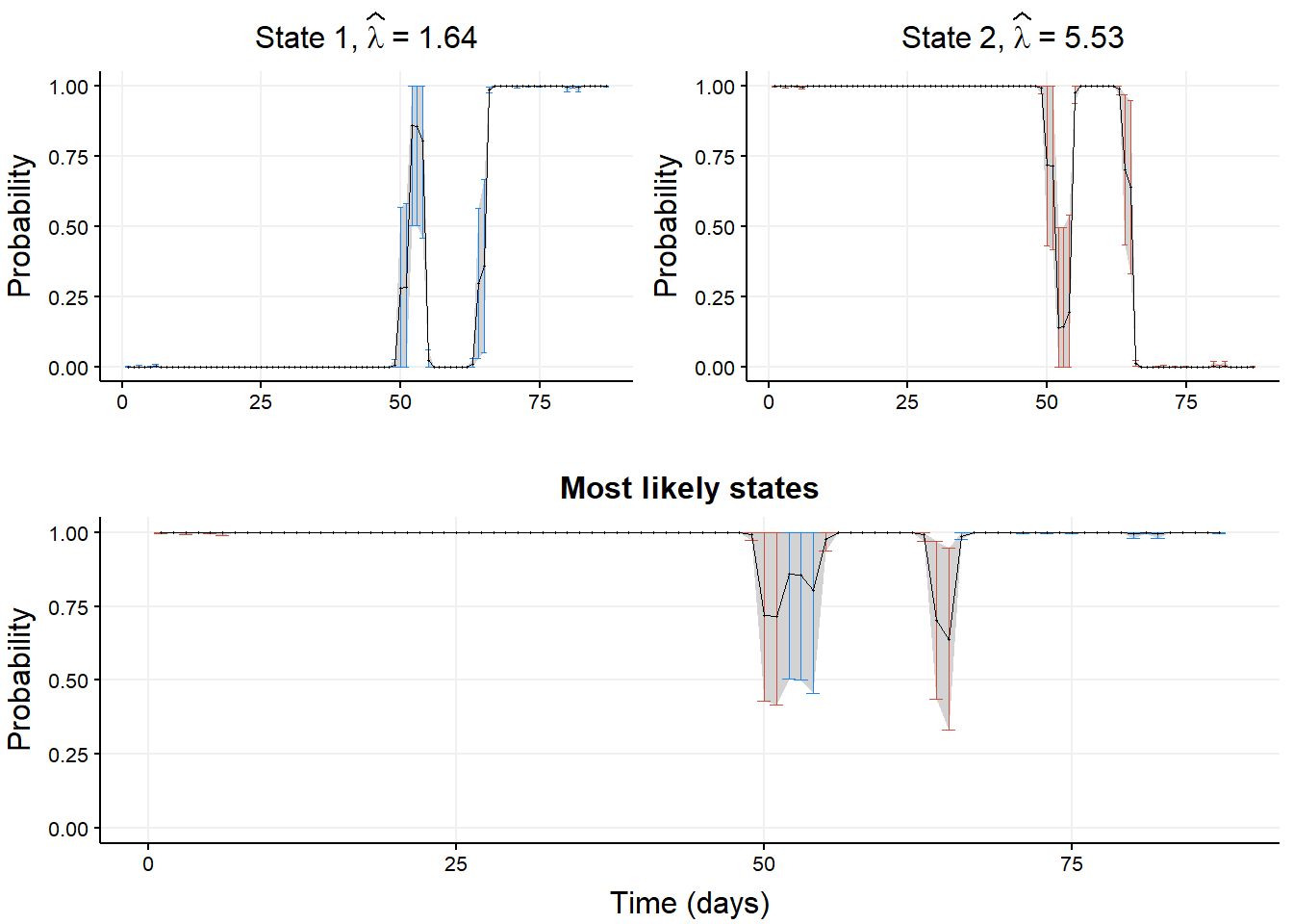
10.4 Limitation
The TYT data set used above is short and does not pose computing issues.
However, with a larger set, retrieving the standard errors of the smoothing probabilities becomes time-consuming and can take days or weeks depending on the dataamount of data, as the delta method is applied repeatedly when these errors are retrieved via summary(sdreport(obj_tmb)).
A solution to this problem is to truncate the smoothing probability matrix before it is returned by TMB, in the objective function defined above.
An example of what the function can be is in the file code/poi_hmm_smoothing_truncated.cpp and below.
#include <TMB.hpp>
#include "../functions/utils.cpp"

// Likelihood for a poisson hidden markov model.
template<class Type>
Type objective_function<Type>::operator() ()
{
  // Data
  DATA_VECTOR(x);          // timeseries vector
  DATA_INTEGER(m);         // Number of states m
  // With a large data set, there are too many smoothing probabilities to return
  // So we truncate them.
  // They are returned as a block of m rows and (size of data set) columns
  // The Eigen library lets us crop that block and return a sub-matrix
  // DATA_INTEGER does not allow for NA, but DATA_SCALAR does, so we use it
  DATA_SCALAR(start_row); // The crop will start with this row index
  DATA_SCALAR(start_col); // The crop will start with this column index
  DATA_SCALAR(nb_rows); // The crop will take this many rows
  DATA_SCALAR(nb_cols); // The crop will take this many columns
  // TODO:
  // Use DATA_UPDATE to adjust the submatrix dimension without reestimating
  // c.f. https://kaskr.github.io/adcomp/group__macros.html#ga3a3716228d46fbe32e23856b2f53be8d

  // Parameters
  PARAMETER_VECTOR(tlambda);     // conditional log_lambdas's
  PARAMETER_VECTOR(tgamma);      // m(m-1) working parameters of TPM

  // Uncomment only when using a non-stationary distribution
  //PARAMETER_VECTOR(tdelta);    // transformed stationary distribution,

  // Transform working parameters to natural parameters:
  vector<Type> lambda = tlambda.exp();
  matrix<Type> gamma = gamma_w2n(m, tgamma);

  // Construct stationary distribution
  vector<Type> delta = stat_dist(m, gamma);
  // If using a non-stationary distribution, use this instead
  //vector<Type> delta = delta_w2n(m, tdelta);

  // Get number of timesteps (n)
  int n = x.size();

  // Are any of these smoothing matrix parameters NA? If yes, set them to the maximum
  int int_start_row, int_start_col, int_nb_rows, int_nb_cols;
  if (start_row != start_row or start_col != start_col or nb_rows != nb_rows or nb_cols != nb_cols) {
    int_start_row = 0;
    int_start_col = 0;
    int_nb_rows = m;
    int_nb_cols = n;
  } else {
    int_start_row = CppAD::Integer(start_row);
    int_start_col = CppAD::Integer(start_col);
    int_nb_rows = CppAD::Integer(nb_rows);
    int_nb_cols = CppAD::Integer(nb_cols);
  }

  // Evaluate conditional distribution: Put conditional
  // probabilities of observed x in n times m matrix
  // (one column for each state, one row for each datapoint):
  matrix<Type> emission_probs(n, m);
  matrix<Type> row1vec(1, m);
  row1vec.setOnes();
  for (int i = 0; i < n; i++) {
    if (x[i] != x[i]) { // f != f returns true if and only if f is NaN.
      // Replace missing values (NA in R, NaN in C++) with 1
      emission_probs.row(i) = row1vec;
    }
    else {
      emission_probs.row(i) = dpois(x[i], lambda, false);
    }
  }

  // Corresponds to (Zucchini et al., 2016, p 333)
  // temp is used in the computation of log-backward probabilities
  matrix<Type> foo, P, temp;
  Type mllk, sumfoo, lscale;

  // Log-forward and log-backward probabilities
  matrix<Type> lalpha(m, n);
  matrix<Type> lbeta(m, n);

  //// Log-forward probabilities (scaling used) and nll computation
  foo.setZero();
  // foo is a matrix where only the first column is relevant (vectors are
  // treated as columns)
  // Specifying "row(0)" or "col(0)" is optional, but it helps to remember
  // if it is a row or a column
  foo = (delta * vector<Type>(emission_probs.row(0))).matrix();
  sumfoo = foo.col(0).sum();
  lscale = log(sumfoo);
  // foo = foo.transpose(); is not reliable because of
  // aliasing, c.f https://eigen.tuxfamily.org/dox/group__TopicAliasing.html
  foo.transposeInPlace();
  // foo is now a matrix where only the first row is relevant.
  foo.row(0) /= sumfoo;
  // We can alternatively use foo.row(0).array().log()
  lalpha.col(0) = vector<Type>(foo.row(0)).log() + lscale;

  for (int i = 2; i <= n; i++) {
    P = emission_probs.row(i - 1);
    foo = ((foo * gamma).array() * P.array()).matrix();
    sumfoo = foo.row(0).sum();
    lscale += log(sumfoo);
    foo.row(0) /= sumfoo;
    lalpha.col(i - 1) = vector<Type>(foo.row(0)).log() + lscale;
  }
  mllk = -lscale;


  //// Log-backward probabilities (scaling used)
  lbeta.setZero();
  // "Type(m)" is used because of a similar issue at
  // https://kaskr.github.io/adcomp/_book/Errors.html#missing-casts-for-vectorized-functions
  foo.row(0).setConstant(1 / Type(m));
  lscale = log(m);
  for (int i = n - 1; i >= 1; i--) {
    P = emission_probs.row(i);
    temp = (P.array() * foo.array()).matrix(); // temp is a row matrix
    // temp must be a column for the matrix product below
    temp.transposeInPlace();
    foo = gamma * temp;
    lbeta.col(i - 1) = foo.col(0).array().log() + lscale;
    // "foo" is a column, but must be turned into a row in order to do
    // the element-wise product above ("P.array() * foo.array()")
    foo.transposeInPlace();
    sumfoo = foo.row(0).sum();
    foo.row(0) /= sumfoo;
    lscale += log(sumfoo);
  }

  //// Local decoding (part 1)
  matrix<Type> smoothing_probs(m, n);
  Type llk = - mllk;
  for (int i = 0; i <= n - 1; i++) {
    if (x[i] != x[i]) {
      // Missing data will get a smoothing probability of NA
      smoothing_probs.col(i).setConstant(x[i]);
    } else {
      smoothing_probs.col(i) = ((lalpha.col(i) + lbeta.col(i)).array() - llk).exp();
    }
  }
  // If there is a large amount of values in smoothing_probs due to e.g. a large
  // amount of data, retrieving submatrices is faster
  // https://eigen.tuxfamily.org/dox/group__QuickRefPage.html
  // block starting at (start_row, start_col) taking nb_rows rows and nb_cols cols
  // If any submatrix parameters are NA, return the entire matrix
  // f != f returns true if and only if f is NaN (NA in R, NaN in C++).
  matrix<Type> truncated_smoothing_probs;
  truncated_smoothing_probs = smoothing_probs.block(int_start_row,
                                                    int_start_col,
                                                    int_nb_rows,
                                                    int_nb_cols);

  // Local decoding (part 2)
  vector<Type> ldecode(int_nb_cols);
  int col_idx;
  for (int i = int_start_row; i < int_start_row + int_nb_cols; i++) {
    // If the data is missing, set the state to -1
    if (x[i] != x[i]) {
      ldecode(i) = x[i];
    } else {
      // https://eigen.tuxfamily.org/dox/group__QuickRefPage.html
      // we don't save the result because we are not interested in the max value
      // only the index
      truncated_smoothing_probs.col(i).maxCoeff(&col_idx);
      // Columns start from 1 in R, but from 0 in C++ so we adjust to be similar
      // to R results.
      ldecode(i) = col_idx + 1;
    }
  }

  // Use adreport on variables for which we want standard errors
  // Be careful, matrices are read column-wise and displayed (like
  // the rest) as part of one vector
  ADREPORT(lambda);
  ADREPORT(gamma);
  ADREPORT(delta);
  ADREPORT(mllk);
  ADREPORT(truncated_smoothing_probs);

  // Variables we need for local decoding and in a convenient format
  REPORT(lambda);
  REPORT(gamma);
  REPORT(delta);
  REPORT(n);
  // REPORT(emission_probs);
  // REPORT(lalpha);
  // REPORT(lbeta);
  // REPORT(smoothing_probs);
  // REPORT(truncated_smoothing_probs);
  REPORT(ldecode);

  return mllk;
}
It is important to note that the values start_row, start_col, nb_rows, and nb_cols cam be set to NA to retrieve the .
They serve to truncate the amount of smoothing probabilities returned, as there are one per combination of data point and hidden state. With 2000 data and 5 hidden states, there will be 10000 smoothing probabilities in a 5 x 2000 matrix.
If needed, one can return all smoothing probabilities by estimating the HMM multiple times and returning each time a different block of the matrix of smoothing probabilities, then aggregating these blocks.
To make use of this, in R, we need to load the modified likelihood function stored in
TMB::compile("code/poi_hmm_smoothing_truncated.cpp")
dyn.load(dynlib("code/poi_hmm_smoothing_truncated"))
.
Then, the TMB_data object can be defined as
TMB_data <- list(x = data_set, m = m,
                 start_row = 0,
                 start_col = 0,
                 nb_rows = m,
                 nb_cols = length(data_set))
or
TMB_data <- list(x = data_set, m = m,
                 start_row = NA,
                 start_col = NA,
                 nb_rows = NA,
                 nb_cols = NA)
and the same smoothing probabilities will be returned as above.
Returning truncated smoothing probabilities can be done as follows
TMB_data <- list(x = data_set, m = m,
start_row = 0, # C++ indexes at 0, unlike R which indexes from 1. Be careful.
start_col = 50, # C++ indexes at 0, unlike R which indexes from 1. Be careful.
nb_rows = m,
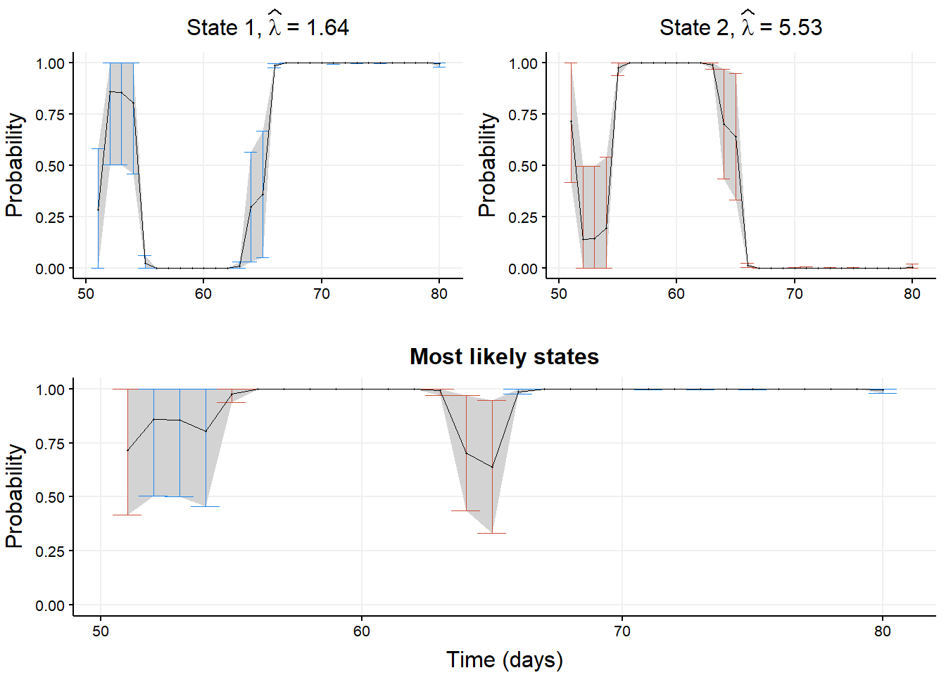
nb_cols = 30). This returns the \(m\) smoothing probabilities associated with data points 51, 52, \(\ldots\), 80.
Remember the updated name of the returned smoothing probabilities from smoothing_probs to truncated_stateprobs for clarity. This will be reflected in the row names of summary(sdreport(obj_tmb)).
Let us show this in action and plot these probabilities as above. We first build the model and retrieve the estimates.
set.seed(1)
# Load TMB, the data set, and utility functions
library(TMB)
source("functions/utils.R")
load("data/tinnitus.RData")
TMB::compile("code/poi_hmm_smoothing_truncated.cpp")
## [1] 0
dyn.load(dynlib("code/poi_hmm_smoothing_truncated"))
m <- 2
data_set <- tinn_data

# Setup initial parameters
lambda <- seq(quantile(data_set, 0.1),
              quantile(data_set, 0.9),
              length.out = m)
gamma <- matrix(0.2 / (m - 1),
                nrow = m,
                ncol = m)
diag(gamma) <- 0.8
delta <- stat.dist(gamma)

# Create the TMB objects for estimation
TMB_data <- list(x = data_set, m = m,
                 start_row = 0,
                 start_col = 50,
                 nb_rows = m,
                 nb_cols = 30)
parameters <- pois.HMM.pn2pw(m, lambda, gamma)

obj_tmb <- MakeADFun(data = TMB_data,
                     parameters = parameters,
                     DLL = "poi_hmm_smoothing_truncated",
                     silent = TRUE)

# Estimation
mod_tmb <- nlminb(start = obj_tmb$par, objective = obj_tmb$fn,
                  gradient = obj_tmb$gr, hessian = obj_tmb$he)

# Retrieve estimates
adrep <- summary(sdreport(obj_tmb))
lambda <- obj_tmb$report(obj_tmb$env$last.par.best)$lambda
gamma <- obj_tmb$report(obj_tmb$env$last.par.best)$gamma

# We are interested only in the smoothing probabilities
adrep <- adrep[rownames(adrep) == "truncated_smoothing_probs", ]

# We follow the notation of (Zucchini et al., 2016)
# One row per hidden state, one column per data
smoothing_probs <- matrix(adrep[, "Estimate"], nrow = m)
smoothing_probs_std_error <- matrix(adrep[, "Std. Error"], nrow = m)
# 95% confidence intervals
q95_norm <- qnorm(1 - 0.05 / 2)
Then we plot the smoothing probabilities and confidence intervals.
# Aesthetic parameters used in the article
ERRORBAR_LINE_WIDTH <- 0.2
ERRORBAR_END_WIDTH <- 1.1
POINT_SIZE <- 0.2
LINE_SIZE <- 0.25
COLORS <- c("dodgerblue2", "tomato3", "green", "purple", "gold")

n <- ncol(smoothing_probs)
indices_to_plot <- 51:80

## Plotting (with ggplot2)
library(ggplot2)

state_ggplot <- list()
for (state in 1:m) {
  # State smoothing probabilities
  stateprobs <- data.frame(idx = indices_to_plot,
                           estimate = smoothing_probs[state, ],
                           std.error = smoothing_probs_std_error[state, ])
  # Add 95% CI bounds with cutoffs at 0 and 1
  stateprobs$ci_lower <- pmax(0, stateprobs$estimate - q95_norm * stateprobs$std.error)
  stateprobs$ci_upper <- pmin(stateprobs$estimate + q95_norm * stateprobs$std.error, 1)

  state_ggplot[[state]] <- ggplot(stateprobs, aes(x = idx)) +
    geom_ribbon(aes(ymin = ci_lower,
                    ymax = ci_upper),
                fill = "lightgrey") +
    geom_errorbar(aes(ymin = ci_lower,
                      ymax = ci_upper,
                      width = ERRORBAR_END_WIDTH),
                  color = COLORS[state],
                  show.legend = FALSE,
                  linewidth = ERRORBAR_LINE_WIDTH) +
    geom_point(aes(y = estimate), size = POINT_SIZE, shape = 16) +
    geom_line(aes(y = estimate), linewidth = LINE_SIZE) +
    ggtitle(bquote("State" ~ .(state) * "," ~ widehat(lambda) ~ "=" ~ .(round(lambda[state], 2)))) +
    theme_Publication() +
    ylim(0, 1) +
    xlab("") +
    ylab("Probability")
}

# STATE MOST LIKELY
ldecode <- obj_tmb$report(obj_tmb$env$last.par.best)$ldecode
ldecode_estimates <- c()
ldecode_std.errors <- c()
for (i in 1:n) {
  ldecode_estimates[i] <- smoothing_probs[ldecode[i], i]
  ldecode_std.errors[i] <- smoothing_probs_std_error[ldecode[i], i]
}
stateprobs <- data.frame(idx = indices_to_plot,
                         estimate = ldecode_estimates,
                         std.error = ldecode_std.errors,
                         state = as.factor(ldecode))
stateprobs$ci_lower <- pmax(0, stateprobs$estimate - q95_norm * stateprobs$std.error)
stateprobs$ci_upper <- pmin(stateprobs$estimate + q95_norm * stateprobs$std.error, 1)

state_likely_ggplot <- ggplot(stateprobs, aes(x = idx)) +
  geom_ribbon(aes(ymin = ci_lower,
                  ymax = ci_upper),
              fill = "lightgrey") +
  geom_errorbar(aes(ymin = ci_lower,
                    ymax = ci_upper,
                    width = ERRORBAR_END_WIDTH,
                    color = state),
                show.legend = FALSE,
                linewidth = ERRORBAR_LINE_WIDTH) +
  geom_point(aes(y = estimate), size = POINT_SIZE) +
  geom_line(aes(y = estimate), linewidth = LINE_SIZE) +
  scale_color_manual(values = COLORS[1:m], breaks = 1:m) +
  ggtitle("Most likely states") +
  theme_Publication() +
  xlab("Time (days)") +
  ylab("Probability") +
  ylim(0, 1)

# Display the graphs in one figure
library(ggpubr)
ggarrange(ggarrange(plotlist = state_ggplot,
                    ncol = 2, nrow = ceiling(m/2)),
          state_likely_ggplot,
          ncol = 1, nrow = 2)